Complexity and Big O Notation

Complexity

Let’s say you have two snippets of code (i.e. algorithms) in front of you. Each snippet performs the same overall function but the implementations are different. If you want to know which one is better in terms of performance/efficiency, the concept of complexity is used.

Complexity is a measure of algorithm performance in terms of the:

execution time (Time Complexity)
required storage space in memory (Space Complexity)
required number of steps or arithmetic operations (Computational Complexity)

In terms of Data Structures and Algorithms, depending on the application, time complexity is typically the priority followed by space complexity. This is because, in modern times, memory is relatively abundant and cheap. Computational complexity is more of a tie-breaker.

Why Complexity?

Why can’t we just run each snippet separately and see which algorithm runs faster? There are a number of reasons for this:

Algorithm performance depends on the input. Algorithms may be faster for certain inputs and slower for others. If we attempt to time code execution with a stopwatch, performance can’t be tested for all possible inputs.
Algorithm performance depends on the hardware/environment in which it is run. Therefore, algorithm runtimes cannot be compared unless ran using the same device with constant conditions for variables like temperature.
Both algorithms would need to be fully implemented in order to test/compare using this method. The chosen language for implementation may also impact results.

Complexity addresses these problems because it provides a way to measure the performance of an algorithm for every possible input regardless of implementation or hardware.

Time Complexity

Time complexity addresses the above issues by summing the number of primitive operations and assuming they all take a constant amount of time. Primitive operations include:

Accesses (i.e. accessing value from an array) -> array[i]
Arithmetic -> x + 5
Assignments -> x = 5
Comparisons -> x < 5
Returns -> return x

Let’s see an example applied to a simple algorithm to find the maximum value in a numerical array:

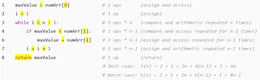
Let’s call the functional relationship between the number of operations required to handle an array t(n) where n is the size of the input array.

In the best case scenario, where the maximum value is at the beginning of the array, line 6 is skipped for every following loop. Therefore, only 4 operations take place in each iteration of the loop. As such:

t(n) = 2 + 1 + 2n + 4(n-1) + 1 = 6n

If we were to graph this relationship, we’d get a straight line with a slope of 6:

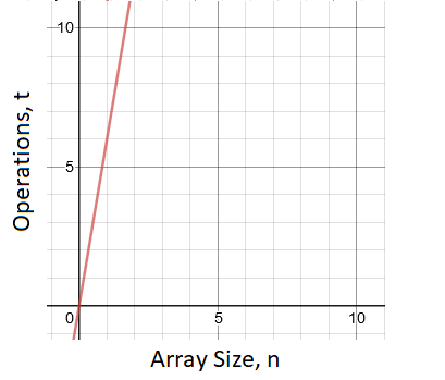
Therefore, for every additional value we add to this array, we’re increasing the execution time by 6 primitive operations. In the worst case scenario, where the maximum value is at the end of the array, line 6 is never skipped. Therefore, 6 operations take place in each iteration of the loop. As a result:

t(n) = 2 + 1 + 2n + 6(n-1) + 1 = 8n-2

In the average case, the maximum value will likely be somewhere in between the first and last element of the array. The resulting performance, therefore, will be somewhere between the best and the worst case.

From this example (more complex examples are to come), you should see how algorithm performance is dependent on the input. In the above example, the size of the input array influenced the execution time of the algorithm. The potential order of numbers within the array resulted in best and worst case execution times. There are 3 notations used to describe these execution times: O, Ω, and Θ.

O (big O): Upper bound on algorithm execution time.
Ω (big omega): Lower bound on algorithm execution time.
Θ (big theta): Both O and Ω simultaneously (unnecessary for tutorial scope).

For practical applications, the main focus is Big O. That’s because the worst case scenario is the most useful piece of information. Efficient algorithms typically use code that has the minimal worst case scenario. However, there are also algorithms where the worst case scenario is statistically unlikely to happen. In these cases, the average runtime should take precedence.

Big O Notation

Now that you have a basic understanding of why complexity is important, let’s look at the most popular method to measure complexity.

Basic Theory

In terms of time complexity, Big O Notation describes how the input size of an algorithm impacts its runtime. In terms of space complexity, Big O Notation describes how the input size of an algorithm impacts its required storage in memory. In other words, it shows how scalable an algorithm is for increasing input sizes. The typical Big O runtime categories are listed with a visualization below:

O(1) - Constant Time
O(log n) - Logarithmic Time
O(n) - Linear Time
O(n log n) - N Log N Time
O(n^p) - Polynomial Time
O(kⁿ) - Exponential Time
O(n!) - Factorial Time

source: bigocheatsheet.com

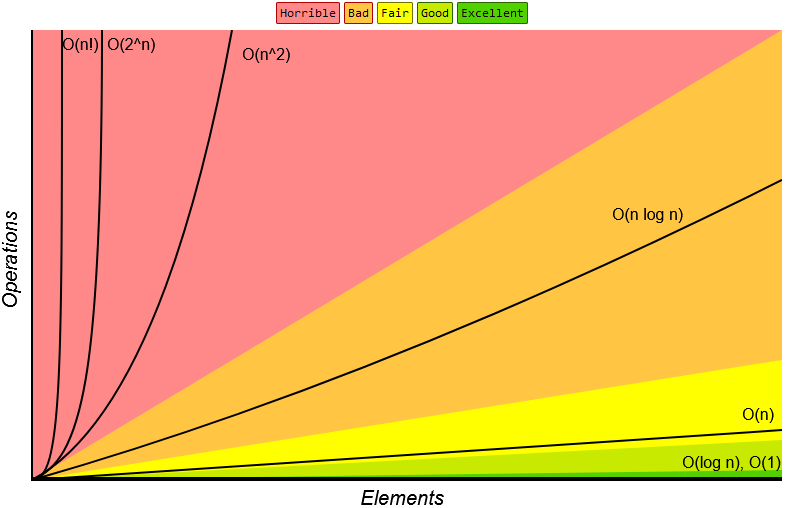
The above image is only meant to show the general shape of the typical Big O functions. At this scale, O(log n) and O(1) appear the same. In reality, O(1) is a horizontal line while O(log n) is a curve that quickly flattens out into a horizontal line. Keep in mind that there are runtimes slower than O(n!). That’s just where the chart cuts off.

Let’s translate these relationships into practical examples. If a code snippet has a “constant” time complexity, it means that, no matter how large the input size is, the same amount of primitive operations will be required to execute the code. Therefore, the runtime will be about the same no matter how large the data input is.

If we have a snippet of code that has a “linear” time complexity. We know that runtime will increase linearly with input size. Recall the previous example from the Time Complexity section:

The Big O (i.e. worst case) runtime is O(8n-2) where n is the size of the input array. You may notice that this is a linear relationship as it follows the linear formula y = mx + b. This expression can be simplified into the O(n) runtime category.

Why do these relationships matter anyway? Well, software developers use them as a means to compare the performance of different algorithms. If we have two algorithms that can sort an array, but the first has a time complexity of O(n log n) and the second has a time complexity of O(n²), we know that the first algorithm will perform much faster for large inputs and is therefore more scalable.

Simple Cases

To get started, let’s derive the Big O time complexity for code commonly seen in simple programs. For your understanding, we’ll start with a couple examples deriving Big O complexity using the longhand/exact method then move to examples using the shorthand/practical method.

Recall that primitive operations include:

Accesses (i.e. accessing value from an array) -> array[i]
Arithmetic -> x + 5
Assignments -> x = 5
Comparisons -> x < 5
Returns -> return x

Disclaimer: My school notes count incrementations such as i++ as 1 operation. Although, it seems like it should be two. Either may be valid depending on who you ask.

The basic steps for calculating Big O time complexity are as follows:

Sum the number of primitive operations line by line
Use the worst case for conditional statements
Simplify the ending expression

Example 1: For loops

Let’s follow the basic steps on the below code snippet:

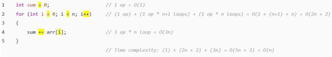
Walking through line by line:

Line 1:
- One operation (assignment) executed once.
Line 2:
- One operation (assignment) executed once.
- One operation (comparison) executed n + 1 times.
  - For example, if i = 3, the conditional would be checked when i = 0, 1, 2, AND 3. Therefore, the condition is executed n + 1 times.
- One operation (incrementation) executed n times (once for every inner loop iteration).
Line 4:
- Three operations (arithmetic, assign, and access) executed n times (once for every inner loop iteration).

Now that we know the complexity of each line, we can sum them into a formula representing the time complexity of the entire algorithm. In this case, we find that the algorithm has a time complexity of O(5n + 3) which is simplified down to O(n).

Why are the constants dropped for simplicity? At large values of n, these constants become relatively insignificant. Realistically, we’re only looking for the simplified Big O notation. That’s where the biggest time savings are found. If you are looking to compare two algorithms that fall under the same Big O category, then you’d keep the constants. However, that’s only really necessary if you want to split hairs over small optimizations.

Example 2: Nested loops

Let’s take it a step further. Instead of one loop, let’s see what happens when we nest two loops together.

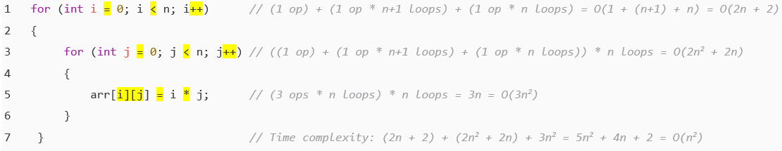
This is similar to the previous example. The twist is that you have to account for the impact of the nesting loops. As we know from the first example, line 1 has a time complexity of O(2n + 2). Line 3, being the exact same type of loop, also has a time complexity of O(2n + 2). However, since line 3 is within a loop, it is executed an additional n times resulting in a complexity of O((2n + 2) * n) = O(2n^2 + 2n). Continuing on, since like 5 performs 3 primitive operations and is nested inside 2 loops, the complexity of line 5 is O(3 * n * n) = O(3n^2). Summing the time complexity of lines 1 through 5 shows us that the overall algorithm has a time complexity of O(5n^2 + 4n + 2) which simplifies to O(n^2).

Example 2.5: Focus on the essentials

You might be thinking, “This process takes forever!”, and you’d be right. Typically, software developers do not calculate time complexities down to the last primitive computation. Practical applications of Big O simplify the final expression at the end anyway. It can be a bit of a pain but knowing the longhand method is important for your understanding. Now that we have that covered, let’s talk about the shorthand method.

For the majority of your time using Big O techniques, you will simply be scanning for the “heavy hitters”, such as loops, on each line and their relationships to each other. Let’s look at the previous example again and take a more streamlined approach. No highlighting necessary.

As you can see, the only important lines to consider were lines 1 and 3. Since we know each loop iterates n times, we know that this compounds into a complexity of O(n²) for the inner loop. That was much faster!

Advanced Cases

The above section explored some fundamental cases. However, as you will find, there are many more advanced cases that require some deeper thinking.

Example 3: Logarithmic complexity

There is a special type of “for” loop that you may come across. Instead of incrementing/decrementing after each iteration, it reduces the remaining iterations by a factor. Here’s an example:

As you can see, instead of incrementing j, the inner for loop divides j by a factor of 2. When an algorithm’s steps are reduced by a factor, the resulting complexity is likely O(log n). Think of it this way. The value of j starts at n and the loop will continue until j falls below 1. With every iteration of the inner loop, the value of j is halved. Therefore, the value of j is converging to a value below 1 at an exponential rate. Inversely, it could be said that the loop’s runtime (or required computations) grows at a logarithmic rate with increasing values of n. Hence the logarithmic O(log n) time complexity.

Example 4: The Sum of Integers 1 through N

Let’s expand our horizons by looking at another special case:

In this example, you will find that the number of iterations of the inner loop depends on the value of i in the outer loop. Initially, when i = 1, the inner loop iterates once. When i = 2, the inner loop iterates twice. This repeats until i = n and the inner loop iterates n times. Therefore, through all values of i, the inner loop executes the sum of 1 + 2 + ... + n times. Mathematically, this sum can be simplified to n(n+1)/2. Therefore, the complexity of the inner loop is O(n²).

Don’t worry if you didn’t already know that simplification. A 10 year old discovered it back in the late 1700s. To be fair, they grew up to be an amazing mathematician and physicist. If you’re not a naturally gifted 10 year old math wizard, you can find an explanation of the proof here.

This pattern appears in software frequently enough that having the formula for the sum of 1 through N memorized is a good idea.

Example 5: Recursive functions

Loops are not the only way lines of code can be compounded multiple times. Recursive functions act in a similar way. Here’s an example function used to calculate the factorial value of an integer:

As you can see, this function will be recursively called until the input value of n is decremented down to 1. Therefore, even though the function itself has a complexity of O(1), it is recursively executed n times. As such, the time complexity is O(1) * n = O(n).

Example 6: Exponential runtimes

In some cases, you will see functions that recursively call themselves multiple times over (the previous example only had one recursive call). Exponential runtimes can result when the end case for a function with multiple recursive calls is approached incrementally rather than exponentially. My favorite example of an exponential runtime comes from Cracking the Coding Interview. The following code returns the nth number of a sequence where every number is double the previous number. For example, the beginning of the sequence is [1, 2, 4, 8, 16, 32, 64, ...]. Therefore, f(4) should yield a result of 8.

In the above algorithm, f(4) will recursively branch off into two f(3) calls. Each f(3) call will branch into two more f(2) calls. This will continue until the f(1) calls end the cycle. This branching is visualized below:

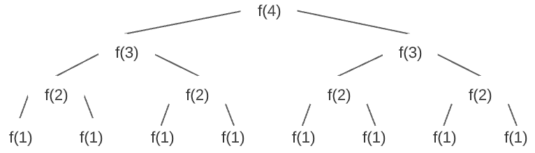
To figure out how many times this O(1) function is recursively executed, we must find the number of nodes in the resulting tree. As can be seen, each iteration doubles the number of nodes. Therefore, we know the complexity is likely exponential because the amount of recursive executions appears to grow at an exponential rate. When dealing with a tree such as this, time complexity can be represented as O(branches^depth) where branches is the number of recursive branches per node and depth is the depth of the tree. In other words, branches is the number of recursive calls within the function and depth is the maximum number of iterations before the input value reaches the end case. Therefore, since there are 2 recursive calls in the function and it takes n iterations for the input value to be decremented to 1, the time complexity of this function is O(2ⁿ).

Another popular example of an algorithm with an exponential runtime is the recursive fibonacci function. It returns the nth number of the fibonacci sequence. For example, the beginning of the fibonacci sequence is [1, 1, 2, 3, 5, 8, 13, ...]. Therefore, fib(4) should yield a result of 3.

In the above algorithm, fib(4) will recursively branch off into a fib(3) call and a fib(2) call. The fib(3) call will branch into a fib(2) call and a fib(1) call. This will continue until the fib(1) and fib(0) calls end the cycle. This branching is visualized below:

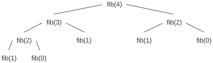
Using the branches^depth equation, the fibonacci method also has a time complexity of O(2ⁿ). However, the recursive fibonacci branching did not create a complete tree like the previous example. That is to say, there are less than 2ⁿ nodes in the above tree. Therefore, the O(1) code snippet is not recursively called exactly 2ⁿ times. If you dive into the math, it’s actually recursively called approximately 1.6ⁿ times. However, 2ⁿ is an acceptable approximation.

Be careful though. In the upcoming sections, you will see that recursive sorting functions like merge sort and quick sort will recursively call themselves twice. However, they will not have exponential time complexities. That’s because the recursive end case is approached at an exponential rate rather than an incremental rate. As a result, the depth component of the O(branches^depth) equation is logarithmic. Therefore, instead of having a time complexity equation resembling O(2ⁿ), the equation is actually O(2^log₂(n)) which, if you know your logarithmic manipulations, is equivalent to O(n).

Complexity Continued

Amortized Time Complexity

Amortized time complexity occurs when an algorithm has different time complexities depending on external conditions. The most common example of this the insertion operation of a dynamic array. When a dynamic array is under capacity, insertions have an O(1) time complexity because new values can be immediately added into the first open index. When a dynamic array is at capacity, it must expand its storage space by creating a new array and duplicating the values over. The additional computations result in an O(n) time complexity since n values of the original array are copied over to a new array. You will see this concept appear again in the data structures section with my sample implementation of a dynamic array.

Space Complexity

Space complexity takes a similar approach to time complexity. However, instead of breaking execution time down into primitive operations of equal value, it breaks storage into primitive spaces of equal value.

When applied to data structures (i.e. computer storage), space complexity accounts for the total number of values stored in memory. For example, an array that stores n values will need O(n) space. Functionally, this means that the required storage space increases linearly with increased array size. Similarly, a 2D array of size n-by-n would require O(n*n) or O(n²) space.

When applied to algorithms (i.e. code snippets), space complexity accounts for the usage of data structures that are dependent on input size. For example, an in-place sort where values are swapped within an existing array will have a space complexity of O(1) since no additional storage that is dependent on input size is required to perform the algorithm. However, an out-of-place sort that involved copying values into a temporary array of size n which would result in an O(n) space complexity. Keep in mind that the existence of additional storage does not inherently increase the space complexity of an algorithm. The size of temporary storage must be impacted by the size of the input. For example, if an algorithm checked an array for its largest 10 values and stored/returned those values in a new array, the algorithm would still have a space complexity of O(1) since the size of the returned array was constant and did not increase with the size of the input array.

When applied to recursive algorithms (i.e. self referential code snippets), space complexity accounts for the memory used up by recursive calls. When a function is executed, an execution context is added to stack memory so that your programming language can track the function’s internal progress and state. Every time a function recursively calls itself, an additional execution context is added to stack memory which takes up space. For example, if a code snippet has an O(1) space complexity (i.e. does not use any additional storage dependent on input size) but is recursively executed n times, then the algorithm may have a space complexity of O(n) since O(1) * n execution contexts = O(n). However, be mindful when considering recursive calls. The previous equation only applies when all n recursive calls exist in stack memory at the same time. For functions that only recursively call themselves a single time, this is typically the case. However, the number of recursive levels (i.e. stack height) does not always match the number of total recursive calls.

For example, if a function recursively calls itself multiple times, its executions can be visualized in a tree-like pattern (see example 6). In this case, instead of all recursive calls existing in stack memory at once, the recursive call stack only gets as high as the depth of the tree. Therefore, as you will see with quick and merge sort, the space complexity of branching recursive functions typically correlates with tree depth. Plenty more examples will be covered in the upcoming sections.

What next?

If this is your first time covering these concepts, the best thing you can do right now is practice. There are plenty of practice resources available for free online. Once you feel up to speed, start the searching algorithms section.