Data Structures
Table of contents:
- Introduction
- Linear Data Structures
- Tree Data Structures
- Hash Data Structures
- Graph Data Structures
- What next?
Introduction
Data structures are methods of organizing data in a computer such that it can be used effectively. Data structures typically fall into 4 general categories:
- Linear (elements arranged sequentially)
- Tree (nodes with hierarchical rules)
- Hash (hash function maps values to keys)
- Graph (nodes without hierarchical rules)
In this section, we will be going over the fundamental data structures belonging to each category. A proper understanding of the fundamental data structures is a necessary stepping stone to understanding more complex data structures. It is also necessary in order to build upon and combine data structures to suit your needs. At the end of this section, you should be able to compare data structures according to their time and space complexities such that you can choose the best structure for a given application.
The time and space complexities of some popular data structures can be seen in the image below:
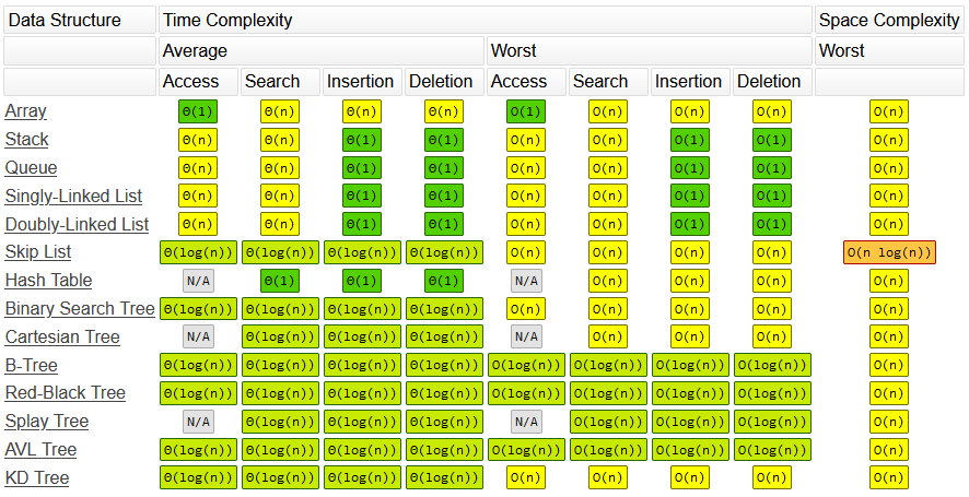
Before moving on, it is important that you know how to interpret the above table. In terms of time complexity, data structures typically have 4 major operations:
- Accessing (AKA indexing): Given an index, find the corresponding value
- Searching: Given a value or key, find a match
- Inserting: Given a value, insert it into the data structure
- Deleting: Given a value or index, delete it from the data structure
Tables like the one above can be really handy. However, they are only truly useful for reviewing data structures that you are already familiar with. Information carried in summaries like this is often overly generalized and dependent on a variety of assumptions.
Critical Thinking
Although the above 4 operations are an essential part of many data structures, they do not apply to everything. For example, you may have noticed that hash tables do not have an “access” operation. This is because some data structures don’t store information sequentially such that every value can be assigned an index. You may have also noticed that some common structures like heaps and graphs are not included on the table. This is because, in many cases, these 4 operations are too general to adequately describe a given data structure.
When using tables found on the internet, it is important to keep in mind that listed values can be misleading. The complexities listed in these tables depend on a variety of assumptions. For example, the O(1) insertion time complexity for linked lists assumes that you already have a reference to the node you’re inserting on. A linked list may have a time complexity of O(1) when inserting at a referenced node such as the head or the tail. However, inserting into the middle of the list requires a sequential search which results in an O(n) runtime. As you can see, vital information can be lost in translation when dealing with simple summaries.
Regarding space complexity, almost all of the fundamental data structures discussed below have an O(n) space complexity where n represents the number of elements or nodes. However, even though many data structures are relatively equivalent in terms of space complexity (i.e. memory scalability), there are situations in which certain data structures outperform others in terms of memory. For example, a densely populated array takes up less space than a linked list of the same size. However, a sparsely populated array takes up more space than a shorter, full linked list.
What To Expect
In this section, we’ll be going over we’ll be going over the fundamental data structures. The format is as follows:
- Brief summary of the data structure.
- Referral to more comprehensive documentation and video tutorials on theory for beginners.
- Referral to my java implementation of the structure.
- Defining the complexities of the major operations of the data structure with reasoning.
- Additional theory where applicable.
I find that the best way to learn how a data structure works is to implement it yourself in your preferred programming language. To serve as examples, I’ve implemented all of the data structures covered in this tutorial using Java. Why Java? It’s more hands-on than Python but not as complex as C++. It’s easy to read and similar in syntax to other popular programming languages. It’s also my first and preferred object-oriented programming language. You can find my Java implementations for each data structures here or in their respective sections.
For additional resources, GeeksForGeeks has extensive documentation on data structures. Including sample implementations in a variety of languages. They also have quizzes and practice questions to assist your learning. Additionally, mycodeschool is a YouTube channel with plenty of high quality video tutorials on data structures. Mycodeschool is an incredible resource for learning data structure theory. Unfortunately, it also has a bit of a tragic backstory and stopped publishing videos back in 2016.
Choosing Data Structures
While you learn about a specific data structure, it is important to understand its performance relative to other data structures. You should be aware of the common applications for a data structure as well as how its complexities cause it to be advantageous or problematic for certain tasks. When you’re choosing a data structure, there are some important questions to ask:
- What data is being stored?
- What are the major operations required by the data structure to store this information?
- What data structures have the lowest complexities for the required operations?
- Can an common data structure adequately handle this responsibility or does a custom data structure need to be made using combinations/specializations of existing data structures?
- Are the benefits of creating a custom data structure worth the required time/effort?
As you learn new data structures, it is important that you can relate them back to the above questions. Ideally, you should know the underlying theory well enough to describe the algorithms (i.e. steps) responsible for their major operations. You should also be able to justify your selection of any particular data structure for a specific application. Try to keep these thoughts in mind.
Linear Data Structures
Linear data structures are the most basic type of data structure. In linear data structures, data is ordered sequentially such that every element is related to their previous and next neighbors by index or reference. To traverse a linear data structure, you move from one element to the next until you reach the end of the line.
Arrays (Dynamic)
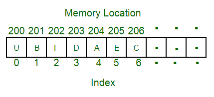
An array is a collection of elements that are stored contiguously (i.e. side-by-side) in memory such that each element can be identified with a corresponding index. Arrays are typically primitive data types so they have little functionality out of the box. In some programming languages, primitive arrays can’t perform common data structure operations such as inserting, and deleting. For clarification, when I say “inserting”, I’m not referring to overwriting an element like arr[0] = 1. I’m referring to inserting a value into a specified index such that no values are overwritten. For example, inserting 3 into [1, 5, 4, 2] such that it becomes [1, 5, 3, 4, 2]. Notice how the index of values 4 and 2 were shifted up by one and still exist in the array. Since primitive arrays can lack these common data structure operations, when “arrays” are compared to other data structures, the comparison typically refers to a “dynamic array” such as an ArrayList or Vector. A dynamic array is essentially just a primitive array that has been extended to perform the common data structure operations as well as dynamically change in size.
Arrays have many applications. As you will find, they are also used implement a variety of other complex data structures. If you’re at the point where you’re learning data structures and algorithms, you likely already know what an array is. If not, refer to the GeeksForGeeks documentation or the mycodeschool video tutorial.
Time and space complexity for array implementations where n is the number of elements:
| Operation | Average/Worst Case | Reasoning |
|---|---|---|
| Indexing | O(1) | Given an index, as you may already know, the corresponding value can be accessed from an array with constant runtime. For example, x = arr[0];. |
| Searching | O(n) | Given a value, an array must be sequentially searched for a match. In the worst case, there is no match and the entire array is traversed. If the array is sorted, a binary search can decrease this complexity to O(log(n)). |
| Inserting | O(n) | If the element is being inserted to the end of the array, the runtime is O(1). In the worst case, the insertion happens at the first index and all elements must be moved up by one index resulting in an O(n) time complexity. For the average case, some fraction of the n elements will be shifted. This simplifies to an O(n) time complexity. |
| Deleting | O(n) | If the element is being deleted from the end of the array, the runtime is O(1). In the worst case, the deletion happens at the first index and all elements must be moved down by one index resulting in an O(n) time complexity. For the average case, some fraction of the n elements will be shifted. This simplifies to an O(n) time complexity. |
| Space Complexity | Reasoning |
|---|---|
| O(n) | An array requires one empty slot for every stored value. |
Note that implementations of dynamic arrays typically increase their size by some factor when they reach capacity. As such, when there is space remaining in the array (i.e. the array is under capacity), insertion to the end of the array is O(1). When there isn’t space and the array must be resized, the time complexity becomes O(n) since n values must be copied into a larger storage array. Since this operation has scenarios that result in different time complexities, it is said to have an amortized time complexity.
Keep in mind that dynamic arrays simply extend primitive arrays and provide the illusion of resizing. Primitive arrays are fixed in size because their data must be physically stored side-by-side in memory such that an index can be established. In reality, resizing a dynamic array involves the copying of n values from a smaller primitive storage array into a larger primitive storage array.
Linked Lists
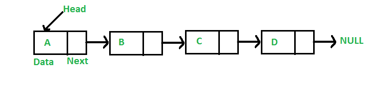
While arrays store data in contiguous memory locations, linked lists store data in contiguous node objects that are connected via pointers/references. All linked lists have a reference to the head (i.e. the first element) like the picture shown above. However, some implementations also have a reference to the tail (i.e. the last element) such that nodes can be quickly added to the end of the list. There are 3 main types of linked lists:
- Singly Linked List (Nodes points to the next node)
- Doubly Linked List (Nodes points to the next and previous node)
- Circular Linked List (Singly or doubly linked list where the tail node points back to the head instead of null)
Linked lists have many applications. Particularly, they are used as lists and to implement a variety of other complex data structures. For more information, see the GeeksForGeeks documentation or the mycodeschool video tutorials.
Time and space complexity for linked list implementations where n is the number of elements:
| Operation | Average/Worst Case | Reasoning |
|---|---|---|
| Indexing | O(n) | Given an index, a linked list must sequentially traverse nodes starting from the head to locate the indexed node. |
| Searching | O(n) | Given a value, a linked list must sequentially search to find a matching value. In the worst case, there is no match and the entire list is traversed. |
| Inserting | O(1) | Assuming insertion involves a referenced node such as the head or tail, it has a constant runtime. However, if you do not have a refence to a node at the desired insertion location, a sequential search is required to find it resulting in an O(n) time complexity. |
| Deleting | O(1) | Assuming deletion involves a referenced node such as the head or tail, it has constant time complexity. However, if you do not have a refence to a node at the desired deletion location, a sequential search is required to find it resulting in an O(n) time complexity. |
| Space Complexity | Reasoning |
|---|---|
| O(n) | A linked list requires one node for every stored value. |
From my example implementations, you may have noticed that arrays and linked lists can perform the same functions. However, their differences provide them with distinct advantages and disadvantages. As such, there are situations where using one over the other is beneficial:
Arrays should generally be used when:
| Situation | Reasoning |
|---|---|
| The number of elements to be stored is known (i.e. array size known) | When arrays are at full capacity, they use less memory than linked lists. |
| Indexing is a major operation | When indexing, arrays have an unbeatable constant time complexity of O(1). Linked lists have a mediocre linear time complexity of O(n). |
Linked lists should generally be used when:
| Situation | Reasoning |
|---|---|
| The number of elements to be stored is unknown | When arrays are below full capacity, they use more memory than linked lists. This is because arrays must be defined at a fixed size. When an array is created, memory corresponding to each element is allocated regardless of whether it is filled with useful data. |
| Constant time insertions/deletions are required | When inserting/deleting around a referenced node such as the head or tail, linked lists have a constant time complexity of O(1). Otherwise, linked lists and arrays both have linear time complexities of O(n). |
Arrays and linked lists are the most important data structures to be familiar with. This is because the other fundamental data structures are implemented using their underlying principles. Make sure you have a good grasp of these data structures before moving on.
Stacks
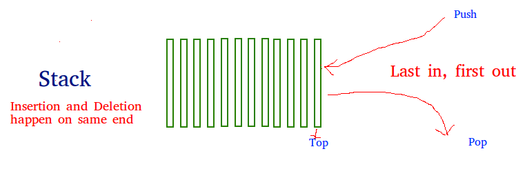
Stacks are what’s known as a LIFO (last in, first out) data structure. Stacks can be visualized as a stack of paper where each piece represents an element stored in the stack. When a element is added to a stack, it is placed on top (i.e. the push() operation). When an element is removed, it is taken from the top (i.e. the pop() operation). As such, the last element to join the stack is the first to leave. Hence the title LIFO.
Stacks have many applications. The most well known is “backtracking” which makes features such as “undo” possible. If you store your previous actions in a stack, they can be easily backtracked. For more information, see the GeeksForGeeks documentation or the mycodeschool video tutorials.
Time and space complexity for stack implementations where n is the number of elements:
| Operation | Average/Worst Case | Reasoning |
|---|---|---|
| Indexing | O(n) | Given an index, a stack must sequentially search itself to locate the corresponding value. This is because stacks aren’t always implemented using an array and the entire purpose of a stack revolves around only accessing the top value. Therefore, get() methods are typically not included. |
| Searching | O(n) | Given a value, a stack must sequentially search itself to locate the corresponding value. |
| Inserting | O(1) | Since stacks always add to the top (an easily indexable location), they have a constant insertion runtime. |
| Deleting | O(1) | Since stacks always remove from the top (an easily indexable location), they have a constant deletion runtime. |
| Space Complexity | Reasoning |
|---|---|
| O(n) | Depending on the implementation, a queue requires one array slot or linked list node for every stored value. |
Queues
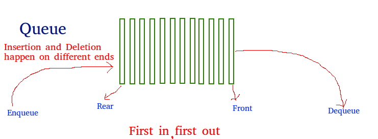
Queues are what’s known as a FIFO (first in, first out) data structure. Queues can be visualized as a line at the grocery store where each person represents an element stored in the queue. When a person joins the queue (i.e the enqueue() operation), they stand at the rear. When a person leaves the queue (i.e. the dequeue() operation), it is from the front. As such, the first person to join the queue is the first person to leave. Hence the title FIFO.
Queues have many applications. They are particularly useful for queuing processes that do not need to be executed immediately. For more information, see the GeeksForGeeks documentation or the mycodeschool video tutorials.
Time and space complexity for queue implementations where n is the number of elements:
| Operation | Average/Worst Case | Reasoning |
|---|---|---|
| Indexing | O(n) | Given an index, a queue must sequentially search itself to locate the corresponding value. This is because queues aren’t always implemented using an array and the entire purpose of a queue revolves around only accessing the front and rear values. Therefore, get() methods are typically not included. |
| Searching | O(n) | Given a value, a queue must sequentially search itself to locate the corresponding value. |
| Inserting | O(1) | Since queues always add to the rear (an easily indexable location), they have a constant insertion runtime. |
| Deleting | O(1) | Since queues always remove from the front (an easily indexable location), they have a constant deletion runtime. |
| Space Complexity | Reasoning |
|---|---|
| O(n) | Depending on the implementation, a queue requires one array slot or linked list node for every stored value. |
Tree Data Structures
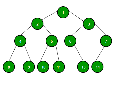
Now that the fundamental linear data structures have been covered, it’s time to look into tree data structures. Binary trees (i.e. trees where nodes have a maximum of 2 children) are the simplest tree data structure. As such, they are useful to cover in terms of understanding tree theory. They are particularly useful at storing hierarchical (i.e. parent/child relation type) data. However, referring to binary trees as a “fundamental data structure” is a bit misleading. Binary trees are not typically used for practical applications. Instead, they are the root to an entire family of more complex/useful data structures such as binary search trees and heaps.
In a tree, each node is called a vertex. The connections between nodes are called edges. The vertex at the very top of a tree is called the root. The vertices at the bottom are called leaf nodes. Vertices refer to each other using parent/child relationship terminology. For example, when a vertex branches down into other vertices, it is referred to as the parent and the branched vertices are referred to as the children. Child vertices of the same parents are siblings, parents of parents are called grandparents, etc. Trees are recursive data structures. That is to say, any given vertex can be considered the root of a subtree. This recursive relationship leads to a lot of interesting software patterns when traversing trees. For more information, see the GeeksForGeeks documentation or the mycodeschool video tutorials.
Tree facts:
- A tree with n vertices (i.e. nodes) has n-1 edges
- Depth: The number of edges between root and chosen node
- Level: Depth + 1 (i.e. the level of the root is 1)
- Height: The number of edges between chosen node a farthest leaf node
- The maximum number of nodes is
branches^depthwherebranchesis the maximum number of children per node anddepthis the maximum depth of the tree (recall that this formula was used in the exponential time complexity section) - A large oak tree can consume about 100 gallons of water per day
Note that, depending on the application, binary trees can be implemented using either arrays or linked lists. Whichever is more efficient/convenient. As you will see, binary search trees are implemented using linked lists while binary heaps are implemented using arrays.
Binary Search Trees (BST)

A binary search tree is an sorted/ordered binary tree. That is to say, for any particular vertex, all children in the left subtree are less than or equal to the value of the vertex and all children in the right subtree are greater than the value of the vertex.
You can think of a linked list as a tree where each node has one parent and one child. The result is a linear chain of nodes. In a binary tree, each node has 2 children (or less) which results in a branched hierarchy of nodes originating from a root. Since data is not stored linearly, trees have distinct advantages as a data structure. For example, binary search trees have significantly better time complexities for search, insertion, and deletion operations than any linear data structure. This is because, instead of sequentially searching themselves to find a value, they only have to traverse a relatively small number of branching edges. If the tree is properly balanced, this traversal is equivalent to performing a binary search which results in an O(log(n)) runtime. Hence the name binary search tree.
A binary tree is considered balanced when the difference in height between the left and right subtrees of each vertex is no more than 1. The height is minimized in a balanced binary tree. If the height is above the minimum, linear sections exist in the tree which limit its ability to efficiently perform a binary search on itself. This is why we want to keep binary trees balanced. Binary search trees can become unbalanced if data is inserted into them in an undesirable order. For example, if the root node happens to be the smallest value in the tree. To fix this problem, several more complex implementations of “self-balancing” binary search trees have been created such as the AVL tree, Red-black tree, and B-tree. However, these are beyond the scope of this tutorial.
For linear data structures, traversal was simple. You just follow the line until you reach the end. For trees, traversal is more complex. Knowing how to traverse a binary tree is an important skill for software interviews. A binary tree can be traversed in any of the following ways:
- Depth-first traversal
- In-order
- Reverse-order
- Pre-order
- Post-order
- Breadth-first traversal
- Level-order
Binary search trees have many applications. They are particularly useful for maintaining a sorted list of data that needs quick/scalable lookup, insertion, and deletion runtimes. For more information, see the GeeksForGeeks documentation or the mycodeschool video tutorials.
Binary Tree Facts:
- Minimum height: log2(n)
- Maximum height: n-1 (i.e. no branching, acts like linked list)
Time and space complexity for binary search tree implementations where n is the number of vertices:
| Operation | Average | Worst | Reasoning |
|---|---|---|---|
| Indexing | O(n) | O(n) | Given an index, a BST must sequentially search itself to locate the corresponding value. Since BSTs are sorted, values can be associated with an index regardless of its branching structure. |
| Searching | O(log(n)) | O(n) | Given a value, a BST must binary search itself for a match. In the worst case, the tree is unbalanced and performs sequential search like a linked list. |
| Inserting | O(log(n)) | O(n) | If the tree is balanced, binary search is used to locate the insertion position. Otherwise, sequential search is used. |
| Deleting | O(log(n)) | O(n) | If the tree is balanced, binary search is used to locate the deletion position. Otherwise, sequential search is used. |
| Space Complexity | Reasoning |
|---|---|
| O(n) | A BST requires one node for every stored value. |
Note that a binary search tree can be implemented using either an array or a series or nodes similar to a linked list. However, arrays are typically reserved for “complete” BSTs where every node is filled due to space limitations.
Binary Heaps
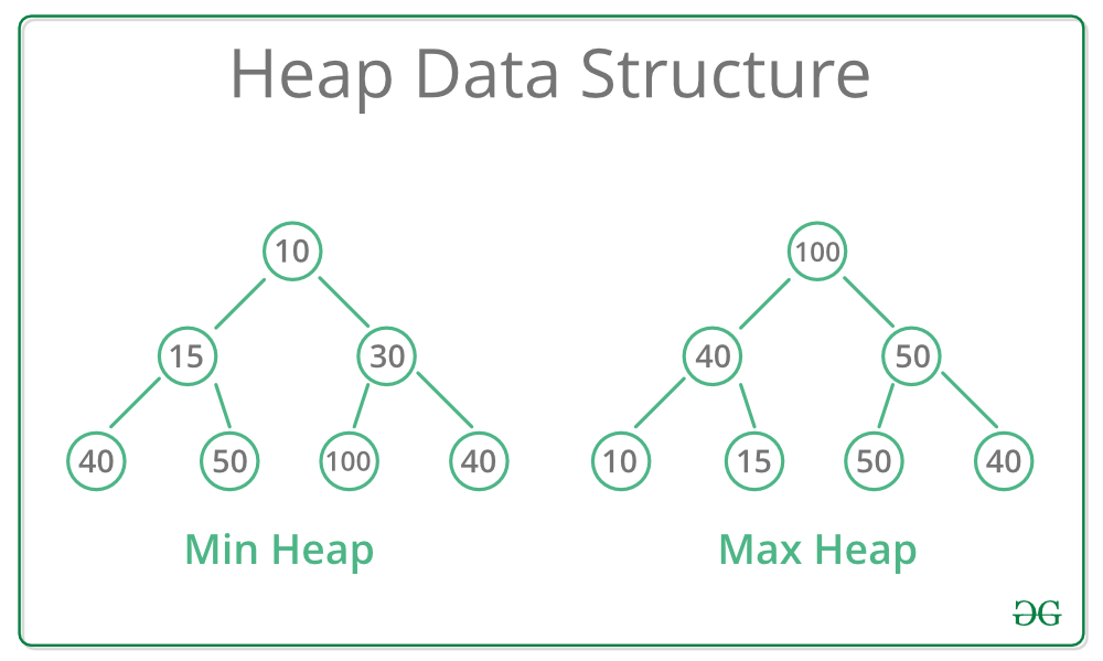
A binary heap is a data structure that stores the maximum or minimum value in the root node of a binary tree (i.e. max and min heaps). A binary heap has the following characteristics:
- For a min heap, all parent nodes must be smaller than their child nodes (vice versa for max heap)
- Insertions take place in order to fill tree levels sequentially from left to right (vice versa for deleting)
Since all parent nodes of the tree must be smaller/larger than their children, the smallest/largest value is always the root of the tree. Additionally, since values are inserted into the binary heap in a specific “left-to-right” order, each node in the tree can be matched with a corresponding index. Since every vertex has an index, binary heaps are best implemented using an array because binary search is not required. This also means that, for any particular node with an index of i:
- The index of the parent is
(i-1)/2 - The index of the left child is
(2*i)+1 - The index of the right child is
(2*i)+2
When inserting into a heap, the new value is placed in the leftmost empty leaf node. For a min heap, if the newly added node is smaller than its parent, it swaps positions with its parents until it reaches the proper position. The process of node swapping is often referred to as “heapifying”. If the root (i.e. the min/max value) is extracted from the heap, the root is replaced with the last leaf node. The relocated leaf node is then “heapified” down the tree to its proper position.
Heaps have many applications. They are particularly useful for implementing priority queues and performing heap sort. For more information, see the GeeksForGeeks documentation or the HackerRank video tutorial.
Time and space complexity for binary heap implementations where n is the number of vertices:
| Operation | Average/Worst Case | Reasoning |
|---|---|---|
| Indexing | O(1) | Given an index, the corresponding value can be accessed in constant time. The min/max value will always be found at index 0 of a min/max heap. |
| Searching | O(n) | Given a value, a heap must sequentially search itself for a match because it is not ordered like a binary tree. |
| Inserting | O(log(n)) | Since a binary heap is always close to a complete/balanced tree, heapifying inserted elements is efficient. |
| Deleting | O(log(n)) | Since a binary heap is always close to a complete/balanced tree, heapifying after deleting elements is efficient. |
| Space Complexity | Reasoning |
|---|---|
| O(n) | A binary heap requires one node for every stored value. |
Hash Data Structures
Hash data structures use a “hash function” to map key-value pairs together such that they can be quickly and conveniently accessed.
Hash Tables
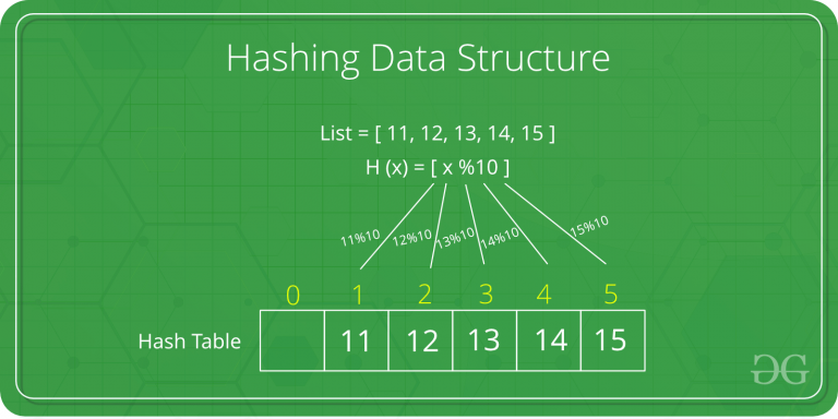
A hash table (AKA hash map) is a data structure used to store key-value pairs. It’s essentially a fancy array where, instead of indexing values with an arbitrary integer, values are indexed with a meaningful “key”. If you’re familiar with Python, you likely already know this data structure to be a dictionary. Hash tables are incredibly useful because, if we know the key, we therefore know the index and can search, insert, and delete with constant runtimes! For this reason, hash tables are probably the most important data structure to master for technical interviews.
So how does it work? Let’s walk through a basic example. Say we want to store a series of employee phone numbers. We could store the phone numbers in an array but it would be practically impossible to remember the index of each phone number if we needed to access it later. We’d have to perform some kind of search on the array which would waste time. Instead, we’ll associate the phone number with the employee’s ID number by:
- Passing the employee ID (i.e. the key) through a “hashing function” that converts the value of their ID to an integer.
- Using that integer as the index position of the phone number (i.e. the value) in the array.
This way, if we want to know an employee’s phone number, we can just pass their ID into the hash table and find it instantly. Pretty cool. There are many ways to implement a hashing function. Many languages have a generic hashing function built in. Choosing the appropriate hash function for the job is a bit of an art in itself.
But wait a second. Even though employee IDs are unique, what if the hashing function returns the same integer for two separate employee IDs? Good question. When two keys yield the same integer for a given hashing function, it is referred to as a “collision”. There are several ways to handle collisions. Some solutions include:
- Separate chaining: Append collided values into the array slot via a linked list
- Open Addressing: Place the collided values in the next empty array slot
- Key selection: If all keys are known ahead of time, a perfect hashing function can be made to prevent collisions.
Although hash tables are implemented using arrays, they are not considered linear data structures because elements don’t have traditional “next” or “previous” neighbors. For a “separate chaining” hash table, each element in the array branches off into a linked list. For “open addressing” hash tables, collided values are placed arbitrarily in the next available index. It’s important to keep this distinction in mind.
Hash tables have many applications. It is particularly useful for solving technical interview questions. For more information, see the GeeksForGeeks documentation or the Paul Programming video tutorial.
Time and space complexity for separate chaining hash table implementations where n is the number of elements:
| Operation | Average | Worst | Reasoning |
|---|---|---|---|
| Searching | O(1) | O(n) | Given a key, if no collisions, accessing the index corresponding to the key is O(1). In a worst case scenario, there are only collisions and searching the linked list is O(n). |
| Inserting | O(1) | O(n) | If no collisions, accessing the index corresponding to the key is O(1) and inserting into the linked list is O(1). In a worst case scenario, there are only collisions and the entire linked list must be traversed to check if the key already exists resulting in an O(n) runtime. |
| Deleting | O(1) | O(n) | If no collisions, accessing the index corresponding to the key is O(1) and deleting from the linked list is O(1). In a worst case scenario, there are only collisions and the entire linked list must be traversed to find the node to be removed resulting in an O(n) runtime. |
| Space Complexity | Reasoning |
|---|---|
| O(n) | A separate chaining hash table needs an array slot and linked list node for each stored value. Regardless, O(2n) simplifies to O(n). |
Note that values are only found in a hash table using a key. Therefore, indexing is not applicable.
Graph Data Structures
As you have seen with binary trees, nodes in a defined hierarchy can from a tree shape. As you will see with graphs, nodes without a defined structure form a web shape. Unlike trees, there are no rules regulating the connection of nodes. Therefore, trees are technically just specialized forms of graph. If that’s true, why are graphs typically covered after hash tables? Well it’s because efficient software implementations of graphs utilize hash tables! Graphs are also much more complex than any of the previous data structures. If you are a math major, you probably already know what a graph is. However, we’ll skip that theoretical jargon for some practical software knowledge.
Graphs
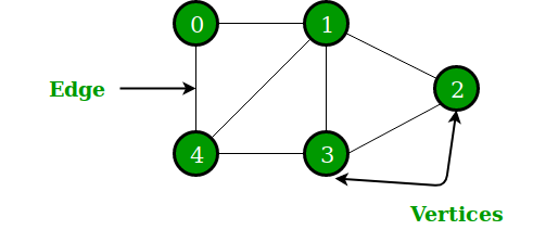
Since a bare-bones graph does not have any rules about connecting nodes, there is a ton of room for specialization. As a result, there are many different types of graphs to cover. If you are learning about graphs for the first time, I highly recommend you check out the mycodeschool video tutorials. I’ve included a summary of related graph theory below.
Graph facts:
- Directed vs Undirected
- Directed graphs (AKA digraphs): Only 1-way edges connect nodes
- Undirected graphs: 2-way edges connect nodes
- Weighted vs Unweighted
- Weighted graphs: Edges have varying values (i.e. weights)
- Unweighted graphs: All edges have the same value
- Simple vs Complex
- Simple graphs: Don’t contain self-edges or multi-edges
- Complex graphs: Contain self-edges and multi-edges
- Self-edge: Edge with only one vertex (i.e. edge connects node to itself)
- Multi-edge: Edge that occurs more than once (i.e. a duplicate edge)
- Dense vs Sparse
- Dense: Number of edges is close to maximum
- Sparse: Number of edges is far from the maximum
Simple graph facts:
- Number of edges for
nnodes- Directed graph: minimum
0, maximumn(n-1) - Undirected graph: minimum
0, maximumn(n-1)/2
- Directed graph: minimum
Connection facts:
- Walk (AKA Path): A sequence of vertices where each adjacent pair is connected by an edge
- Disclaimer: When people say “path”, they’re typically referring to a “simple path” rather than a “walk”
- Walk types
- Simple Path: A walk where no nodes (and therefore edges) are repeatedly visited
- Trail: A walk where no edges are repeatedly visited
- Closed walk: A walk that starts and ends on the same node
- Cycle (AKA simple cycle): A closed walk where the only repetition is the start/end.
- A graph is considered “connected” if there is a path from any vertex to any other vertex.
- If a directed graph is considered “connected”, it is also considered “strongly connected”
- If a directed graph is not “strongly connected” but would become so if it had 2-way edges, then it is considered “weakly connected”
- A graph is considered “acyclic” if it has no cycle (i.e. cannot traverse from a node back to itself without repetition).
A graph can be implemented with an “adjacency matrix” or an “adjacency list. Adjacency matrices are used for dense graphs where the number of edges approaches the maximum (i.e. all nodes connect to almost all other nodes). Conversely, adjacency lists are used for sparse graphs where there are relatively few edges per node (most real world graphs are sparse).
Graphs have many applications. They are particular useful for relating data in a web-like formation. For example, web pages in the World Wide Web or users in a social media site. Graphs are also used to make search engines and road mapping software. For more information, see the GeeksForGeeks documentation.
Time and space complexity for adjacency matrix graph implementations where |V| is the number of vertices and |E| is the number of edges:
| Operation | Average/Worst Case | Reasoning |
|---|---|---|
| Adding a vertex | O(|V|2) | To increase the size of the storage matrix, a new, larger matrix (i.e. 2D array) must be created and all values must be copied over. |
| Removing a vertex | O(|V|2) | To decrease the size of the storage matrix, a new, smaller matrix (i.e. 2D array) must be created and all values must be copied over. |
| Adding an edge | O(1) | To add an edge, the value in matrix[i][j] must be set to from 0 to 1 (or the appropriate weight value). Where i is the index of the first vertex and j is the index of the second vertex. |
| Removing an edge | O(1) | To remove an edge, the value in matrix[i][j] must be set to from 1 (or the weighted value) to 0. Where i is the index of the first vertex and j is the index of the second vertex. |
| Checking if two vertices connect | O(1) | A connection can be confirmed by checking that matrix[i][j] is not zero. Where i is the index of the first vertex and j is the index of the second vertex. |
| Space Complexity | Reasoning |
|---|---|
| O(|V|2) | If there are |V| vertices, a |V|x|V| matrix is required for storage. |
Time and space complexity for adjacency list graph implementations where |V| is the number of vertices and |E| is the number of edges:
| Operation | Average/Worst Case | Reasoning |
|---|---|---|
| Adding a vertex | O(1) | Assuming a hash table is used to store adjacency lists, a new vertex can be created in constant time. If not, a search must be performed to check if the vertex already exists resulting in O(|V|) time. |
| Removing a vertex | O(|V| + |E|) | In order for a vertex to be removed, it must be removed from every adjacency list. Traversing to every vertex in the hash table is O(|V|) and traversing every adjacency list (i.e. every edge) is O(|E|). |
| Adding an edge | O(1) | To add an edge, a vertex must be added to the appropriate adjacency list. Finding the adjacency list from the hash table is O(1). Inserting the vertex into the adjacency list (i.e. linked list) is O(1). This process is repeated twice for non-directional edges. |
| Removing an edge | O(|V|) | To remove an edge, a vertex must be removed from the appropriate adjacency list. Finding the adjacency list from the hash table is O(1). Traversing the adjacency list for a match is O(|V|) because, in the worst case, all vertices are in the adjacency list. Removing the vertex from the adjacency list (i.e. linked list) is O(1). This process is repeated twice for non-directional edges. |
| Checking if two vertices connect | O(|V|) | Finding the adjacency list of the first vertex using the hash table is O(1). Traversing the adjacency list for a match of the second vertex is O(|V|) because, in the worst case, all vertices are in the adjacency list. Removing the vertex from the adjacency list (i.e. linked list) is O(1). |
| Space Complexity | Reasoning |
|---|---|
| O(|V|2) | For each edge, an additional vertex is stored. Two for a non-direction edge. |
What next?
There’s one more data structure that I will be adding to this page eventually. It’s called a trie and can also be very helpful for technical interviews. If you’re applying to large tech companies, you should probably learn this data structure.
Knowing about the fundamental data structures is just a baseline. As you continue to improve as a software developer, you will likely apply these data structures in conjunction to create even more complex/specialized data structures to suit your needs. The sky’s the limit! If this is your first time covering these concepts, it might take some time for things to really sink in. In my opinion, the best thing you can do is implement the above data structures yourself in your preferred programming language. When you are comfortable, check out the next section.