Sorting Algorithms
Table of contents:
Introduction
Sorting is the arrangement of elements within a collection into increasing or decreasing order of some property. There are many scenarios where a developer may want a collection sorted. One of the biggest advantages of having a sorted collection is that you can utilize binary search which can make an algorithm significantly more scalable/efficient. Now that you are familiar with the fundamental data structures, it’s time to learn the fundamental array sorting algorithms. Why arrays? Well, arrays are the most simple/common type of data structure. More complex data structures are often implemented using arrays. Therefore, knowing how to sort an array is an important skill.
Technically, under the right conditions, these sorting algorithms can be applied to any linear data structure. Therefore, when you are learning these algorithms, it is important to focus on understanding the general process instead of memorizing the exact implementation. That way, you can apply them to other linear data structures in any language regardless of the underlying conditions.
You may be wondering why this section is being covered after data structures. The reason is that some complex sorting algorithms utilize complex data structures. For example, stacks are sometimes used to implement an iterative version of quick sort. Additionally, binary heaps are used to implement heap sort.
There are a great deal of sorting algorithms out there:
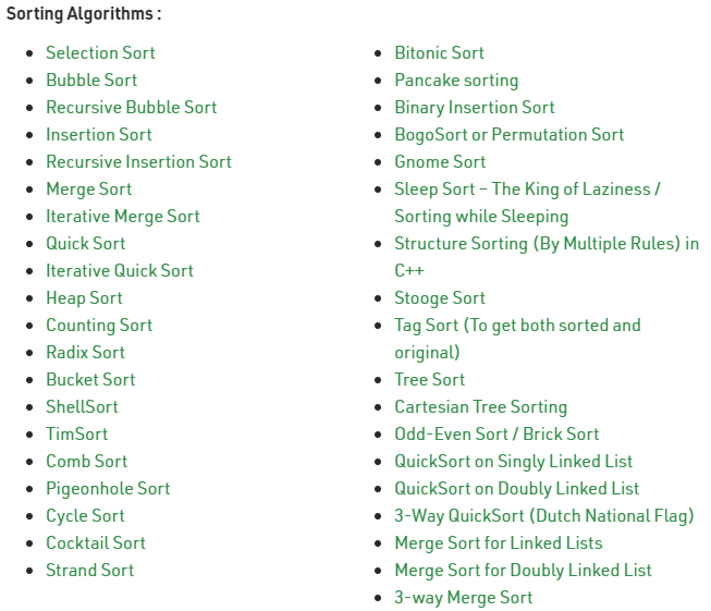
However, we’ll just be learning about the fundamental algorithms you would likely see in a university or junior interview environment. We’ll start with the most basic sorting algorithms:
- Selection sort
- Bubble sort
- Insertion sort
Then we’ll cover some more useful/advanced sorting algorithms:
- Merge sort
- Quick sort (random)
- More to be added later…
If you want to empirically see how the performance of these sorting algorithms compare, I have implemented them in Java. Using this script, you can record the runtime of each sorting algorithm with input arrays of varying orders and sizes.
I find that the best way to learn sorting algorithms is to implement them yourself in your preferred programming language. If you are a visual learner, a great tool you can use is visualgo.net. This website allows you to visualize various sorting algorithms on custom arrays. You can go at your own pace working step-by-step through the code. Another good resource is GeeksForGeeks. Their website contains implementations of each sorting algorithm in a variety of programming languages. If you like videos, mycodeschool is a YouTube channel with plenty of high quality video tutorials on sorting algorithms.
Background
Before moving on, you should be familiar with the following sorting terminology:
| Term | Definition |
|---|---|
| in-place sort | A sort that swaps data within a data structure without the help of additional data structures for temporary storage. We want our sorting algorithms to be in-place wherever possible because it minimizes space complexity. |
| stable sort | A sort that preserves the relative order of equivalent elements. That is to say, if two elements of equal (primary key) value exist in a certain order before sorting, they will remain in the same order after sorting. |
| internal sort | A sort where data is kept in primary memory (i.e. in RAM using arrays) |
| external sort | A sort where data is kept in secondary memory (i.e. on disk or tape) |
In addition to the above terminology, sorting algorithms can also be labelled as either “recursive” or “non-recursive” depending on whether their implementations use recursion. For more information on sorting theory, see the mycodeschool video tutorial.
Basic Sorting Algorithms
The time and space complexities of common array sorting algorithms are shown below:
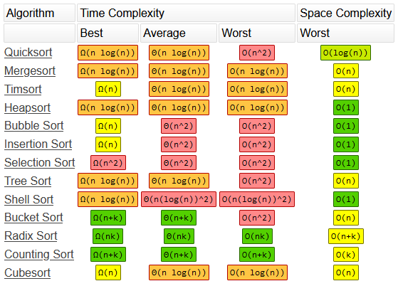
From the above chart, using your Big O knowledge, you should be able to tell that the basic sorting algorithms of bubble, insertion, and selection sort are not very scalable due to their O(n^2) average/worst case runtimes. However, this doesn’t mean they are useless. The basic sorting algorithms are simple to learn and implement. Therefore, they are a good place to start when learning about sorting algorithms. Although they are not scalable for large collections, they are perfectly reasonable to use when sorting relatively small collections. In some cases, they may be more beneficial to use due to their simplicity and ease of implementation.
Selection Sort

Description
Selection sort is often related to sorting a hand of playing cards. The algorithm is as follows:
- Start with all the cards in your right hand (i.e. the unsorted subarray shown above in blue).
- Select the minimum card from your right hand and place it into the end of your left hand (i.e. the sorted subarray shown above in orange).
- Repeat until all cards have moved from your unsorted right hand to your sorted left hand.
The above algorithm can be implemented using two separate arrays (sorted and unsorted). However, that would make the space complexity of the algorithm O(n). Ideally, we want our sorting algorithms to be in-place with constant O(1) space complexity if possible. Therefore, instead of using 2 arrays, we can simply swap elements around to create sorted/unsorted subsections within the original array. For more information, see the mycodeschool video tutorial.
Implementation in Java
Complexity
Time complexity of selection sort where n is the number of elements:
| All cases | Reasoning |
|---|---|
| O(n2) | For every element in the array, the unsorted subarray must be sequentially searched for the minimum value. An O(n) search repeated n times results in an O(n^2) runtime. If the array is already sorted, this process still takes place. |
Space complexity of selection sort where n is the number of elements:
| All cases | Reasoning |
|---|---|
| O(1) | All memory allocations are constant space (in-place sort) and no recursive calls are made. |
Bubble Sort
Description
The bubble sort algorithm steps through the array and swaps an element with its neighbor if it is out of order. This way, the largest unsorted value “bubbles” to the to end of the array on each pass. Since we know that the largest value has been properly sorted (shown above in orange), additional passes are performed using the remaining, unsorted subsection of the array (shown above in blue). Optimized versions of bubble sort also break from the loop if the array is detected to be sorted. For more information, see the mycodeschool video tutorial.
Implementation in Java
Complexity
Time complexity of bubble sort where n is the number of elements:
| Best | Average/Worst | Reasoning |
|---|---|---|
| O(n) | O(n2) | In the best case, the array is already sorted and bubble sort only traverses once. In the average/worst case, the array is in random/descending order and an O(n) traversal occurs for a portion of or all of the n elements. |
Space complexity of insertion sort where n is the number of elements:
| All cases | Reasoning |
|---|---|
| O(1) | All memory allocations are constant space (in-place sort) and no recursive calls are made. |
Insertion Sort
Description
Insertion sort is the last and most efficient of the 3 basic sorting algorithms. Similar to selection sort, insertion sort can be visualized with a deck of playing cards:
- Start with all the cards in your right hand. (i.e. unsorted subarray shown above in blue).
- Select a card and place it into your left hand into the proper sorted position. (i.e. sorted subarray shown above in orange).
- Repeat until all cards have moved from your unsorted right hand to your sorted left hand.
In terms of software implementation, to remove a card from the unsorted subarray, you simply:
- Store the first element of the unsorted array in a temporary variable (shown above in red).
- Increment the index of its previous neighbors in the sorted subarray until the correct insertion index is made vacant.
- Insert the stored element into the vacant, sorted position.
For more information, see the mycodeschool video tutorial.
Implementation in Java
Complexity
Time complexity of insertion sort where n is the number of elements:
| Best | Average/Worst | Reasoning |
|---|---|---|
| O(n) | O(n2) | In the best case, the array is already sorted and insertion sort only traverses once. In the worst case, the array is in descending order and an O(n) neighbor incrementation occurs for every element in the array (i.e. n times). |
Space complexity of insertion sort where n is the number of elements:
| All cases | Reasoning |
|---|---|
| O(1) | All memory allocations are constant space (in-place sort) and no recursive calls are made. |
Advanced Sorting Algorithms
The above sorting algorithms can be handy in very basic scenarios involving small collection. However, to sort larger data structures, we’re going to need something a little more comprehensive. The following sorting algorithms are must more efficient/scalable.
Merge Sort
Description
In the previous sorting algorithms, the array was sorted by dividing the array into “sorted” and “unsorted” subsections. Merge sort takes a different approach because it is a recursive algorithm. An overly simplified approximation of the recursive algorithm can be described like so:
- Split the array in half
- Sort the two smaller arrays
- Merge the two sorted smaller arrays back into a single sorted array
The above algorithm is overly simplistic because recursion actually removes the need for the second step. Since the algorithm is recursive, the array is actually divided until there are n subarrays that consist of a single element. This can be seen in the above gif when every element starts as a different color. Since a subarray of one element is already sorted, each subarray is then recursively merged back together in sorted order. A good visualization of this process can be seen here:
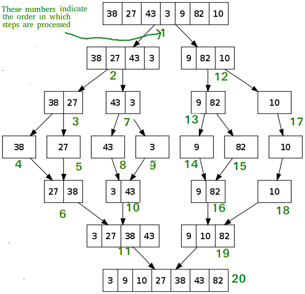
The order in which elements are split and merged back together is indicated by the green numbers. The order of the merging process is best visualized in the above gif. Merge sort is a stable sorting algorithm. For more information, see the mycodeschool video tutorial.
Implementation in Java
Complexity
Time complexity of merge sort where n is the number of elements:
| All cases | Reasoning |
|---|---|
| O(n log2(n)) | Since merge sort divides the array by a factor of 2 in every recursive step, division until subarrays are a single element in length will take log(n) recursive levels. In each recursive level, n values are sequentially traversed when copying/merging subarrays. |
Space complexity of insertion sort where n is the number of elements:
| All cases | Reasoning |
|---|---|
| O(n) | Merge sort has a space complexity of O(n) because it is not an in-place sort. When merging, the two sorted subarray halves are copied into temporary arrays (of collective size n on the first recursive level) and then combined back into the original array in sorted order. |
Quick Sort (Random)
Description
Similar to merge sort, quick sort is recursive. Unlike merge sort, quick sort is a non-stable, in-place sorting algorithm which gives it an advantage in terms of space complexity. You may notice that it has a worst case time complexity of O(n^2). However, this case is almost never seen using “randomized” quick sort where the “pivot” is selected at random. Quick sort is actually such a practical choice for an efficient sorting algorithm that programming libraries typically implement it for generic sorting functions. The algorithm is as follows:
- Select a random element to be the pivot and swap to last (or first, as seen in the above gif) index position.
- Define a partition index and rearrange the list such that all elements lesser than the pivot (shown in green) are to the left of the partition index and all elements greater than the pivot (shown in purple) are to the right (doesn’t have to be sorted).
- Swap the pivot from the last (or first) index to the partition index. The pivot is now sorted (shown in orange).
- Recursively repeat the above process on the unsorted subarrays to the left and right of the pivot until the entire array is sorted.
For more information, see the mycodeschool video tutorial.
Implementation in Java
Complexity
Time complexity of quick sort where n is the number of elements:
| Best/Average | Worst | Reasoning |
|---|---|---|
| O(n log2(n)) | O(n2) | In the best/average case, partitioning is balanced such that left and right subarrays are of relatively equal size. This way, quick sort divides the array by some factor on each recursive step. As such, division until we have reached a single element will take approximately log(n) recursive levels. On each recursive level, the remaining (i.e. some factor of n) elements are sequentially traversed when arranging around the partition index. In the worst case, partitioning is always unbalanced (i.e. the pivot is always the largest/smallest element in the array) and only left/right subarrays are created during the recursive process. Therefore, division until we have reached a single element will take n recursive levels (resembling a linked list). This case is statistically improbable when the pivot is selected at random. |
Space complexity of insertion sort where n is the number of elements:
| Best/Average | Worst | Reasoning |
|---|---|---|
| O(log2(n)) | O(n) | Quick sort is an in-place sort and therefore does not require the use of temporary data structures. However, since it is a recursive algorithm, additional space is required to account for the data stored on each recursive level. That is why the space complexity corresponds with time complexity in this case. In the best/average case there are log(n) recursive levels with O(1) space complexity and log(n) * O(1) = O(log(n)). In the worst case, there are n recursive levels with O(1) space complexity and n * O(1) = O(n). |
What next?
There are many more sorting algorithms. I will add more such as heap, radix, and counting sort to this page eventually. The rest is up to you as you face more specialized software problems. If you want to empirically see how the performance of these sorting algorithms compare, using this script, you can record the runtime of each sorting algorithm with input arrays of varying orders and sizes. When you are comfortable with this section, check out the next section.